3D Poisson Equation
Background
Let ![]() be a bounded, simply or multiply connected domain in
be a bounded, simply or multiply connected domain in  with a Lipschitz boundary
  The Poisson equation for a scalar function
 ![]() in
in  is given by
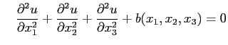
where ![]() represents a source function prescribed on
represents a source function prescribed on ![]() .
.
A solution ![]() of the Poisson equation admits an integral representation, known as the Green's representation formula, expressed as
of the Poisson equation admits an integral representation, known as the Green's representation formula, expressed as

where ![]() is the unit normal to
is the unit normal to ![]() directed towards the exterior of
directed towards the exterior of ![]()
![]() is the flux associated with the function
is the flux associated with the function![]() and the kernels
and the kernels ![]() and
and ![]() are given respectively by
are given respectively by
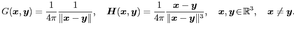
Here ![]() is the usual Euclidean norm in
is the usual Euclidean norm in ![]() defined as
defined as ![]() . In addition, it was established in [1] that the Newton potential admits a boundary representation as
. In addition, it was established in [1] that the Newton potential admits a boundary representation as
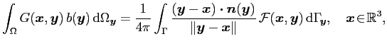
where
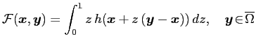
with![]() denoting an extension of the source function
denoting an extension of the source function ![]() into any ball centered at
into any ball centered at ![]() and containing
and containing ![]() . In particular, a continuation
. In particular, a continuation ![]() of the source function
of the source function ![]() can be specified as
can be specified as
This representation of the Newton potential in term of surface integral allows a numerical solution of the Poisson equation that does not require a volume-fitted mesh.
Solution via a boundary element method
To approximately solve the Poisson equation via a Boundary Element Method (BEM), the surface ![]() is usually discretized into flat triangles
is usually discretized into flat triangles ![]() using a mesh generation software (e.g. CUBIT).
using a mesh generation software (e.g. CUBIT).
![\includegraphics[height=1.5in]{ct896g}](/Imgs/ImgLaplace/img21.png)
With reference to [1], the functions ![]() and
and ![]() are assumed to have a polynomial variation over each triangle (boundary element)
are assumed to have a polynomial variation over each triangle (boundary element)![]()
Approaches:
Galerkin BEM
References
- [1] S. Nintcheu Fata.
Treatment of domain integrals in boundary element methods.
Appl. Num. Math., 62(6):720-735, 2012.