3D Lame Equation
Background
Let ![]() be a bounded, simply or multiply connected, domain in
be a bounded, simply or multiply connected, domain in  with Lipschitz boundary
 ![]() occupying a homogeneous isotropic elastic solid that is characterized by the Lamé parameters
occupying a homogeneous isotropic elastic solid that is characterized by the Lamé parameters ![]() and
and ![]() In linear elasticity, the Lamé equation which describes the static equilibrium of a deformable body in terms of the displacement vector
In linear elasticity, the Lamé equation which describes the static equilibrium of a deformable body in terms of the displacement vector ![]() is defined as
is defined as
where ![]() represents a body force prescribed on
represents a body force prescribed on ![]() To deal with the Lamé equation, let where
To deal with the Lamé equation, let where ![]() be the unit normal to
be the unit normal to ![]() directed towards the exterior of
directed towards the exterior of ![]() and let
and let ![]() be the traction vector on
be the traction vector on ![]() associated with the displacement
associated with the displacement ![]() where the stress tensor
where the stress tensor![]() is introduced as
is introduced as
with ![]() denoting the symmetric second-order identity tensor on
denoting the symmetric second-order identity tensor on ![]() and the superscript "
and the superscript "![]() " representing the transpose symbol. A solution
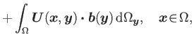
" representing the transpose symbol. A solution ![]() of the Lamé equation admits an integral representation, known as the Somigliana identity, expressed as
of the Lamé equation admits an integral representation, known as the Somigliana identity, expressed as
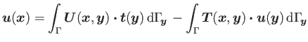
where the kernels ![]() and
and ![]() are given respectively as
are given respectively as

and
![$\displaystyle \frac{-1}{8\pi(1-\nu)}\frac{1}{\Vert\boldsymbol{x}-\boldsymbol{y}...
...mbol{x}-\boldsymbol{y})}{\Vert\boldsymbol{x}-\boldsymbol{y}\Vert}\right]\right.$](/Imgs/ImgLame/lam_img25.png)
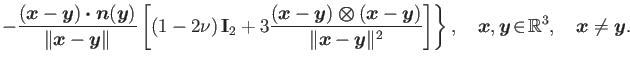
Here the elastic constant ![]() is called the Poisson ratio of the solid
is called the Poisson ratio of the solid ![]() and
and![]() is the usual Euclidean norm in
is the usual Euclidean norm in ![]() defined as
defined as ![]() . Moreover, it was established in [2] that the Newton potential admits a boundary representation as
. Moreover, it was established in [2] that the Newton potential admits a boundary representation as
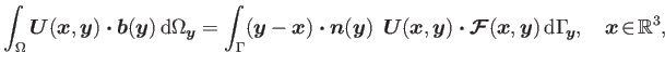
where
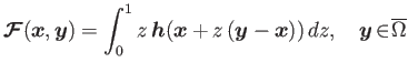
with ![]() denoting an extension of the body force
denoting an extension of the body force ![]() into any ball centered at
into any ball centered at ![]() and containing
and containing ![]() . In particular, a continuation
. In particular, a continuation ![]() of the body force
of the body force ![]() can be specified as
can be specified as
This representation of the elastic Newton potential in term of surface integral allows a numerical solution of the Lamé equation that does not require a volume-fitted mesh.
Solution via a boundary element method
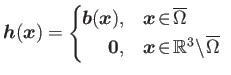
To approximately solve the Lamé equation via a Boundary Element Method (BEM), the surface ![]() is usually discretized into flat triangles
is usually discretized into flat triangles ![]() using a mesh generation software (e.g. CUBIT).
using a mesh generation software (e.g. CUBIT).
![\includegraphics[height=1.5in]{ct896g}](/Imgs/ImgLaplace/img21.png)
With reference to [1], the vector fields ![]() and
and ![]() are assumed to have a polynomial variation over each triangle (boundary element)
are assumed to have a polynomial variation over each triangle (boundary element)![]()
Approaches:
Galerkin BEM
References
- [1] S. Nintcheu Fata.
Explicit expressions for three-dimensional boundary integrals in linear elasticity.
J. Comput. Appl. Math., 235(15):4480-4495, 2011. - [2] S. Nintcheu Fata.
Boundary integral approximation of volume potentials in three-dimensional linear elasticity.
J. Comput. Appl. Math., 242(1):275-284, 2013.