Collocation BEM for 3D Laplace Equation
Download CBEM_LAP, a package for solving the 3D Laplace equation based on a piecewise constant Collocation Boundary Element Method.
Piecewise constant collocation method
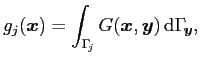
The potential ![]() and flux
and flux ![]() are assumed to be constant over each boundary element. It can be shown (see cbem_lapGuide.pdf provided in the package CBEM_LAP) that the potentials
are assumed to be constant over each boundary element. It can be shown (see cbem_lapGuide.pdf provided in the package CBEM_LAP) that the potentials
 and
and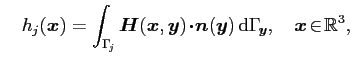
due to a uniform source distribution over a flat triangle ![]() can be employed to successfully compute
can be employed to successfully compute ![]() and
and ![]() on
on ![]() . In addition, these potentials can be utilized to effectively calculate
. In addition, these potentials can be utilized to effectively calculate ![]() at interior points
at interior points ![]() The analytic expressions for
The analytic expressions for![]() and
and![]() over a flat triangle are given in [1].
over a flat triangle are given in [1].
References
- [1] S. Nintcheu Fata.
Explicit expressions for 3D boundary integrals in potential theory.
Int. J. Num. Meth. Eng., 78(1):32-47, 2009.